Tuesday, December 31, 2024

Monkey Dog Problem - Grid Multiplication

The following problems was recently posted in the IIM-Cal puzzle group (and eventually in my puzzle group as well): Can we fill an $n \times n$ grid with the first $n^2$ integers such that the product of the numbers in the $k$th row equals that of the $k$th column for $1 \leq k \leq n$?

The fact that this is impossible for $n=2$ is easy to show by inspection. Vamshi Jandhyala in our group posted grids with the required property for $3 \times 3$ and $4 \times 4$ (and eventually for $10 \times 10$) using a Python non-linear solver. However, this approach ended up time-expensive for larger grids.

He also showed such grids are impossible whenever $n=9$ or $n>10$ using a nice argument involving the number of primes between $n^2/2$ and $n^2$.

Not wanting to get into the realm of non-linearity, I log'ed the entire grid so that multiplication becomes addition and the problem becomes linear. Note that this made an Integer Non-Linear problem to a Non-Integer Linear problem. Despite precision errors, this approach worked for $n=3,4$ but proved elusive for larger $n$.

Running out of options, I eventually realised that each grid that satisfies the required property can be seen only for a particular prime (their exponents in all the $n^2$ numbers to be specific) while ignoring others.


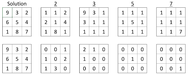
The top half of the above snapshot shows a solution to a $3 \times 3$ grid for a particular prime. The bottom half shows the same but in terms of the exponents of the prime.

The prime exponents form makes it clear that the problem can indeed be modelled as an Integer Linear Problem which can be solved extremely efficiently using free solvers in Python. In fact, doing so enables us to solve the problem for all the cases in a matter of seconds.

A Solution for $5 \times 5$ grid

A Solution for $6 \times 6$ grid

A Solution for $7 \times 7$ grid

A Solution for $8 \times 8$ grid

Python code used for solving this problem.

from ortools.linear_solver import pywraplp
import numpy as np


def main():
    # Data
    n = 3
    vals = []
    # primes = [2, 3, 5, 7, 11, 13, 17, 19, 23]
    # primes = [2, 3, 5, 7, 11, 13, 17, 19, 23, 29, 31, 37, 41, 43, 47]
    # primes = [2, 3, 5, 7, 11, 13, 17, 19, 23, 29, 31, 37, 41, 43, 47, 53, 59, 61]
    primes = [2, 3, 5, 7]
    primepi = len(primes)
    
    def vals(i0, k):
        i, cnt, p = i0, 0, primes[k]
        while i % p == 0:
            i //= p
            cnt += 1
        return cnt

    # Solver
    # Create the mip solver with the SCIP backend.
    solver = pywraplp.Solver.CreateSolver("SCIP")

    x = {}
    for i in range(n * n):
        for j in range(n * n):
            x[i, j] = solver.IntVar(0, 1, "")
    
    for i in range(n * n):
        solver.Add(solver.Sum([x[i, j] for j in range(n * n)]) == 1)
    
    for j in range(n * n):
        solver.Add(solver.Sum([x[i, j] for i in range(n * n)]) == 1)
    
    y = {}
    for i in range(n * n):
        for k in range(primepi):
            y[i, k] = solver.Sum([x[i, j] * vals(j + 1, k) for j in range(n * n)])

    
    rowsum = {}
    for i in range(n):
        for k in range(primepi):
            rowsum[i, k] = solver.Sum([y[j, k] for j in range(n * i, n * i + n)])
    
    colsum = {}
    for i in range(n):
        for k in range(primepi):
            colsum[i, k] = solver.Sum([y[j, k] for j in range(i, n * n, n)])
    
    for i in range(n):
        for k in range(primepi):
            solver.Add(rowsum[i, k] == colsum[i, k])
    
    solver.Minimize(1)
    status = solver.Solve()

    # Print solution.
    if status == pywraplp.Solver.OPTIMAL or status == pywraplp.Solver.FEASIBLE:
        res = []
        for i in range(n * n):
            for j in range(n * n):
                if x[i, j].solution_value() > 0:
                    res += [j + 1]
        print(res)
    else:
        print("No solution found.")


if __name__ == "__main__":
    main()

That eventually settles the Monkey Dog Problem of Grid multiplication. There is also an interesting question of finding $n$ which has the lowest number of solutions if rotations and reflections are identified. That could be left as an exercise to the reader.

Hope you enjoyed this. See ya later.

Until then
Yours Aye
Me

Saturday, November 30, 2024

Five ways of solving an Expected Value problem

 Let's say an Independent Aurelian is investigating butterflies on two types of traits, A and B. It is known that the probability of a butterfly exhibiting trait A is $p$ and that of trait B is $q$ (independent of each other). Note that this means the probability of a butterfly exhibiting both these traits is $pq$.

If she wants to study both these traits, how many butterflies, on average, would she need to catch? She can do this either by catching two butterflies each with exactly on of these traits or by catching a butterfly with both these traits.

The problem is simple and that subject of this post is look at five different methods of this problem. A key fact that will be of great use in all these methods is that for an event with success probability $r$, we would need, on average, $1/r$ trials to get the first success.

Simple equation

Let $N$ be the expected value we are looking for. We can condition this based on the nature of the first butterfly that is caught.

$\displaystyle N=(1-p)(1-q)\cdot(1+N)+(1-p)q\cdot \left(1+\frac{1}{p}\right)+p(1-q)\cdot\left(1+\frac{1}{q}\right)+pq\cdot 1$

Transfer Matrix

It is easy to setup the transfer matrix for this problem with the states being $\{\text{None, Only trait }A\text{, Only trait }B\text{, Both}\}$. Then the transfer matrix $\mathbf{T}$ is,

$\displaystyle \mathbf{T}=\begin{pmatrix}1-(1-p)(1-q)&p(1-q)&(1-p)q&pq \\ 0&1-q&0&q \\ 0&0&1-p&p \\ 0&0&0&1\end{pmatrix}$

It is then well known that the expected value is given by $\mathbf{1}(\mathbf{I}-\mathbf{T})^{-1}$ where $\mathbf{I}$ is the identity matrix and $\mathbf{1}$ is a row matrix of 1's.

Infinite Series

Let's say we've caught $n$ butterflies. The probability that none of them have trait A is $(1-p)^n$ which means that atleast one of them have trait A is $1-(1-p)^n$ and the same applies for trait B as well (with $p$ replaced with $q$).

$\mathbb{P}(\text{atleast of one each of both traits in }n\text{ trials})=(1-(1-p)^n)(1-(1-q)^n)$

With this, we see that $\mathbb{P}(N>n)=1-(1-(1-p)^n)(1-(1-q)^n)$

Then, $\displaystyle \mathbb{E}(N)=\sum_{n=0}^\infty \mathbb{P}(N>n)=\sum_{n=0}^\infty \Bigl (1-(1-(1-p)^n)(1-(1-q)^n) \Bigl )$

Story proof

We can answer this more directly. The expected number of butterflies needed can be broken into parts. First, expected number to get atleast one of the traits and second, the remaining value.

The probability of a butterfly exhibiting one of the traits is $1-(1-p)(1-q)=p(1-q)+(1-p)q+pq$. Therefore, we would need $1/(1-(1-p)(1-q))$ trials to get atleast of the traits. Now,

$\displaystyle \mathbb{P}(\text{Only trait A}|\text{atleast one of the traits})=\frac{p(1-q)}{p(1-q)+(1-p)q+pq}=\frac{p(1-q)}{1-(1-p)(1-q)}$

After having got trait A, we would be looking for trait B which we would get, on average, in $1/q$ trails. This approach applies for the other two cases as well. Therefore,

$\displaystyle\mathbb{E}(N)=\frac{1}{1-(1-p)(1-q)}+\frac{p(1-q)}{1-(1-p)(1-q)}\cdot\frac{1}{q}+\frac{(1-p)q}{1-(1-p)(1-q)}\cdot\frac{1}{p}+\frac{pq}{1-(1-p)(1-q)}\cdot 0$

(Shorter story proof using) Min-Max identity

It is easy to see that $x_1+x_2=\max (x_1,x_2)+\min (x_1,x_2)$ for any two real $x_1,x_2$.

Using this and the linearity of expectations, we have,

$\mathbb{E}(N)=\mathbb{E}(\text{trials to get trait A})+\mathbb{E}(\text{trials to get trait B})-\mathbb{E}(\text{trials to get atleast one of the traits})$

All of these are Geometric random variables with probabilities $p$, $q$ and $p+q-pq$. Therefore,

$\displaystyle \mathbb{E}(N)=\frac{1}{p}+\frac{1}{q}-\frac{1}{p+q-pq}$


Where's the fun in solving a problem if getting an answer is the only objective?

Yours Aye
Me

A Geometric Optimisation problem

Consider two circles $A(B)$ and $C(B)$ intersecting at $B$ and $D$, and a line passing through $D$. Let this line intersect the circle $A(B)$ at $F$ and the circle $C(B)$ at $G$.

The question of maximising the arithmetic mean of $DF$ and $DG$ is well known. It is also known that Euclidean construction of the line that maximises the Harmonic mean of $DF$ and $DG$ is impossible. We already saw the construction of the line that maximises the Geometric mean of $DF$ and $DG$ in this blog.

In this post we are interested in constructing the line such that the Quadratic mean of $DF$ and $DG$ is maximised. In fact, we solve a slightly more general problem. For a given $\theta$, we construct the line such that $\sqrt{DF^2+DG^2-2 \cdot DF \cdot DG \cdot \cos \theta}$ is maximised.

We first use some auxiliary points and lines that helps us in the final solution. For a given $\theta$, construct points $D'$ and $D'_1$ such that $\angle DAD'=\angle DCD'_1=\theta$. Construct the circle that passes through $D$, $B$ and $D'_1$.

For any point $E$ on this circle, let the line $ED'$ intersect circle $A(B)$ at $F$. Let $G$ be likewise on circle $C(B)$. Construct line $FG$. We first show that the line $FG$ passes through $D$.

We know that $\angle FD'B+\angle FDB=\pi$ because they are opposite angles in a cyclic quadrilateral. But $\angle FD'B=\angle ED'B=\pi-\angle ED'_1B$ because $\angle ED'B$ and $\angle ED'_1B$ are opposite angles of a cyclic quadrilateral. Now, $\angle FD'B=\angle BD'_1G=\angle BDG$.

Therefore, $\angle BDG + \angle FDB=\pi$ which shows that $F$, $D$ and $G$ are collinear.

Now, by construction, $\theta / 2=\angle D'BD=\angle D'_1BD$ and therefore, $\angle D'BD'_1=\theta$. This shows that $\angle D'ED'_1=\pi-\theta$.

We know that $\angle DGD'_1=\angle DBD'_1=\theta/2$ because they are angles in a same segment of a circle. Because $\angle DAD'=\theta$, we can see that $\angle DFD'=\pi-\theta/2$, and therefore $\angle DFE=\theta/2$.

Thus we have shown that $\triangle FEG$ is isosceles with $FE=EG$. Therefore, we can quickly see that $FG=2EF\cos(\theta/2)$.

Using Stewart's theorem on this triangle for the cevian DE, we have,

$EF^2=DE^2+DF\cdot DG$

Multiplying by $(2\cos(\theta/2))^2$ on both sides and simplifying, we get

$(2\cos(\theta/2))^2DE^2=FG^2-2DF\cdot DG \cdot 2\cos^2(\theta/2)$

Using the fact that $FG=DF+DG$ and $\cos\theta=2\cos^2(\theta/2)-1$,

$(2\cos(\theta/2))^2DE^2=DF^2+DG^2-2\cdot DF \cdot DG \cdot \cos\theta$

As $\theta$ is given, the above expression shows that maximising the RHS amounts to maximising $DE$. But this can be easily achieved. We just draw the line joining $D$ and center of circle $D'BD'_1$. The point at which this line intersects the circle gives us $E$ from which we can trivially construct the line $FG$ using what we've described before.

Hope you enjoyed this. See ya soon.

Until then, Yours Aye

Me

Tuesday, September 3, 2024

An Odd Sum

Someone in our puzzle group recently posted a question which asked to evaluate the following sum.

$$\frac{1}{e^{\pi}+1}+\frac{3}{e^{3\pi}+1}+\frac{5}{e^{5\pi}+1}+\cdots$$

My first instinct was to check the sum with Wolfram Alpha which showed me that this sum equals $1/24$. This made me curious.

I recast the sum into the following form.

$$\frac{e^{-\pi}}{1+e^{-\pi}}+\frac{3e^{-3\pi}}{1+e^{-3\pi}}+\frac{5e^{-5\pi}}{1+e^{5\pi}}+\cdots$$

The individual terms reminded me of Lambert series which eventually led me into rabbit hole that is to be the content of this post.

Let's define the following function $f(q)$ such that

$\displaystyle f(q)=\frac{q}{1+q}+\frac{3q^3}{1+q^3}+\frac{5q^5}{1+q^5}+\cdots$

Then,

$\displaystyle -f(-q)=\frac{q}{1-q}+\frac{3q^3}{1-q^3}+\frac{5q^5}{1-q^5}+\cdots$

Expanding using the lambert series for divisor functions, we see

$\displaystyle -f(-q)=\sigma_{\text{odd}}(1)q+\sigma_{\text{odd}}(2)q^2+\sigma_{\text{odd}}(3)q^3+\cdots=\sum_n \sigma_{\text{odd}}(n)q^n$

where $\sigma_{\text{odd}}(n)$ where is sum-of-odd-divisors function.

The sum-of-odd-divisors functions is intimately tied to the number of representations of an integer by a sum of four squares (Jacobi four square theorem) and by sum of four triangular numbers (Legendre). See Analogues on two classical theorems on representations of a number and The Parents of Jacobi’s Four Squares Theorem Are Unique, for example.

Therefore,

$\begin{align}
\displaystyle -f(-q) &= \sum_n \sigma_{\text{odd}}(n)q^n \\ &=\frac{1}{24} \left[8\sum_{n\text{ odd}}\sigma_{\text{odd}}(n)q^n + 24\sum_{n\text{ even}}\sigma_{\text{odd}}(n)q^n + 16\sum_{n\text{ odd}}\sigma_{\text{odd}}(n)q^n \right] \\ &= \frac{1}{24}\left(\sum_n r_4(n)q^n+\sum_n t_4(n) q^n \right) \\ &= \frac{\vartheta_2(q)^4+\vartheta_3(q)^4-1}{24}\end{align}$

where $r_4(n)$ (and $t_4(n)$) is the sum-of-four-squares (and sum-of-four-triangulars) function, and $\vartheta_3(q)$ (and $\vartheta_2(q)$) is the third (and second) Jacobi elliptic function.

It is well known that

$\displaystyle \vartheta_3(q)=\sum_{n=-\infty}^\infty q^{n^2}=\phi(q^2)\prod_{n \text{ odd}}(1+q^n)^2$ and 

$\displaystyle \vartheta_2(q)=\sum_{n=-\infty}^\infty q^{(n+1/2)^2}=2\phi(q^2)q^{1/4}\prod_{n \text{ even}}(1+q^n)^2$

where $\displaystyle\phi(q)=\prod_{n}(1-q^n)$ is the Euler function.

Note that

$\displaystyle \prod_{n\text{ odd}}(1-q^n)=\frac{\phi(q)}{\phi(q^2)}$ and $\displaystyle \prod_{n}(1+q^n)=\frac{\phi(q^2)}{\phi(q)}$

Therefore,

$\displaystyle \vartheta_3(-q)=\phi(q^2)\frac{\phi(q)}{\phi(q^2)}\frac{\phi(q)}{\phi(q^2)}$ and $\displaystyle \vartheta_2(-q)=2\phi(q^2)(-q)^{1/4}\frac{\phi(q^4)}{\phi(q^2)}\frac{\phi(q^4)}{\phi(q^2)}$

Now,

$\displaystyle\sqrt\frac{\vartheta_2(-q)}{\vartheta_3(-q)}=\sqrt{2}(-q)^{1/8}\frac{\phi(q^4)}{\phi(q)}$

Putting $q=e^{-\pi}$ in the above expression, we have

$\displaystyle\sqrt\frac{\vartheta_2(-e^{-\pi})}{\vartheta_3(-e^{-\pi})}=\sqrt{2}(-1)^{1/8}e^{-\pi/8}\frac{\phi(e^{-4\pi})}{\phi(e^{-\pi})}$

Using the special values of the Euler function, we see that $\displaystyle \phi(e^{-4\pi})=\frac{e^{\pi/8}}{\sqrt{2}}\phi(e^{-\pi})$

Then,

$\displaystyle\sqrt\frac{\vartheta_2(-e^{-\pi})}{\vartheta_3(-e^{-\pi})}=(-1)^{1/8} \implies \vartheta_2(-e^{-\pi})^4+\vartheta_3(-e^{-\pi})^4=0$

Returning to our expression for $f(q)$, we see that $24f(e^{-\pi})=1-\vartheta_2(-e^{-\pi})^4-\vartheta_3(-e^{-\pi})^4=1$

As $f(e^{-\pi})$ is essentially the sum that we started with, we finally see that

$$\displaystyle\frac{1}{e^{\pi}+1}+\frac{3}{e^{3\pi}+1}+\frac{5}{e^{5\pi}+1}+\cdots=\frac{1}{24}$$

Phew!

As an aside, we could probably arrive the result a little quicker by using some results like

$\displaystyle\lambda(-1+i)=\frac{\vartheta_2(e^{(-1+i)\pi})^4}{\vartheta_3(e^{(-1+i)\pi})^4}=\frac{\vartheta_2(-e^{-\pi})^4}{\vartheta_3(-e^{-\pi})^4}=-1$ (or) $G_1=1\text{ and }g_1=2^{-1/8}$

where $\lambda(n)$ is the Modular lambda function and $g\text{ and }G$ are the Ramanujan g- and G- functions. But I didn't want to bring in additional exotic functions into the problem especially when I can't find a source for the above values of these functions.


Hope you enjoyed this. See ya soon.

Until then, Yours Aye

Me

Monday, July 1, 2024

Tautochronous tanks

Toricelli's law states that the velocity of a discharge, say $v$, located at the bottom of a tank filled to a height $h$ is $v=\sqrt{2gh}$.

Assuming the shape of the tank to be a right prism (with its axis along the $y$-axis), we can use the conservation of mass (or volume in this context) to get

$A \,dy=-a \cdot \sqrt{2gy}\,dt$

where $A$ is the cross sectional area of the prism and $a$ is the area of discharge. Note that the negative sign indicates that $y$ (the height of the water column) decreases as time $t$ increases.

Rearranging and integrating, we have

$\displaystyle \int_0^T \,dt=-\frac{A}{a\sqrt{2g}}\int_h^0 \frac{1}{\sqrt{y}}\,dy \implies T=\frac{A}{a}\sqrt{\frac{2h}{g}}$

where $T$ is the total time taken to drain the tank which is proportional to the square root of the height of the liquid column.

But can we design a tank such that the time of discharge is directly proportional to height? If we assume that the shape of the tank is a solid of revolution such that the area of the cross section at $y$ is given by $A(y)$, then by the similar reasoning as above, we have

$\displaystyle T=\frac{1}{a\sqrt{2g}}\int_0^h \frac{A(y)}{\sqrt{y}}\,dy$

Therefore, for $A(y)=\pi x^2 \propto \sqrt{y}$ (or) $x \propto \sqrt[4]{y}$, we get that $T(h)$ is directly proportional to $h$.

This clearly shows that the draining time for a tank formed by the solid of revolution quartic curve $y=x^4$ is directly proportional to height of the liquid column.

This naturally leads to the second question that we want to address in this post. Can we design a tank such that the draining time is independent of the height of the liquid column.

A direct attack (for example, using Abel's solution of the Tautochrone curve) quickly suggests that there is no such curve.

This might seem like a dead end and it sort of is. But, Let's consider an almost similar question: Can we design a tank, initially filled to the brim, such that the time of discharge is independent of the height at which the discharging hole is located?

For ease of what follows, we orient the coordinate system such that gravity points in the positive $y$ direction. Then for a tank whose shape is a solid of revolution, using the conservation of volume, we have,

$\displaystyle A(y)\,dy=a\cdot \sqrt{2g(y_0-y)}\,dt \implies T(y_0)=\frac{1}{a\sqrt{2g}}\int_0^{y_0}\frac{A(y)}{\sqrt{y_0-y}}\,dy$

where $y_0$ is the height at which the discharge is located.

Now, if we use Abel's idea, we can see that

$\displaystyle A(y)=T_0\frac{a\sqrt{2g}}{\pi}\frac{1}{\sqrt{y}}$

And there we have it! The inverse quartic equation $y=x^{-4}$ is tautochronous such that the time taken to empty the tank is independent of the 'depth' of the water column.

Because the $x$-axis is asymptotic to the inverse quartic curve, we should also ensure that the tank holds a finite volume of water of water for a given height of discharge. But it's an easy exercise to check that the volume is indeed finite.

Hope you enjoyed this. See ya soon.

Until then, Yours Aye

Me

Saturday, May 18, 2024

A nice Geometric Optimisation Problem - Part 2

This post picks up where we left earlier.

In addition to the centre of circumcircle of $\triangle KDL$, the midpoint of the segment $KL$ also lies in the circle. In fact, this can be proved more easily.

Let $A$ and $C$ be the centers of the respective circles. It can be easily seen that $2\angle CAD=\angle BAD=2\angle BQD=2\angle BKD$ which means $\angle CAD=\angle BKD$. Similarly, we can show that $\angle ACD=\angle BLD$. Hence, we see that $\triangle ACD \sim \triangle KLD$.

If we let $O$ be the midpoint of $AC$ and $P$ be the midpoint of $KL$, then by the similarity of the triangle we established before, we have $\angle DOC=\angle DPL=\angle DPB$. Because $\angle DOC$ is constant, we see that $P$ subtends a constant angle with segment $BD$ and hence lies on a circle containing $B$ and $D$.

Also, note that $\angle BOD=2\angle DOC=2\angle DPB=2\angle DSB$ where $S$ is as shown below. Because the angle subtended by $O$ with segment $BD$ is twice that of $P$, we know that $O$ is the center of circle containing $P$.

As both $J$ and $O$ lie on the perpendicular bisector of $AC$ at the product-maximising-position, segment $DT$ (where $T$ is shown below) is parallel to $AC$. Also, $\angle BDT$ is right angled which makes $BT$ the diameter of $P$'s locus.

Because $\angle NDT$ is right angle, we see that $NT$, which is the perpendicular bisector of $KL$ at the product-maximising position, is the diameter of $\triangle KLD$'s circumcircle.

We know that $\angle KTN=\angle KDN$ and $\angle LDN=\angle LTN$ (angles subtended by the same chord in a circle), we see that $\angle KDB=\angle LDB$.

Therefore, we finally see that at the product-maximising position, $ND$ (or) $BD$ should be the angle bisector $\angle KDB$ which is the relation we were looking for in the previous post.

Hope you enjoyed this. See ya later.

Until then
Yours Aye
Me

A nice Geometric Optimisation Problem - Part I

Consider two circles of different radii intersecting at $B$ and $D$. If we now draw a line $KL$ through $B$ as shown in the following figure, the question of determining the position at which the sum of $BK$ and $BL$ maximised is one of the famous non trivial problems in Geometric Optimisation.

We can solve this by noting that $\triangle KDL$ remains self similar. Because both $\angle BKD$ and $\angle BLD$ are angles subtended by the same chord $BD$ in the respective circles, the angles in the triangle remain constant irrespective of the position of the line $KL$. 

 Therefore $KL$ will be maximised when $DK$ (or $DL$) is as large as possible which happens when they are the respective diameters of the given circles. We could also see that, at this position $KL$ and $BD$ will be perpendicular to each other.

A natural follow up question would be find the position of $KL$ such that the product of $BK$ and $BL$ is maximised. Find a geometric construction of the position along with a geometric proof for the same proved more challenging that I had anticipated. That proof will be the subject of this post.

Before I start, I also want to point out that the proof here may seem unnecessarily complicated. But if anyone can share the shorter and elegant geometric proof for this problem, I would be really grateful.

To begin with, if we construct the circle passing through $K$, $D$ and $L$, and extend the segment $BD$ so that it intersects the circumcircle at $N$, then by the power-of-the-point theorem, we know that

$BK \cdot BL = BD \cdot BN$

Therefore, maximising the product of $BK$ and $BL$ is the same as maximising $BD \cdot BN$. But $BD$ is a constant independent of the position of the segment $KL$. Hence, the problem we are after reduces to that of maximising the segment $BN$ or $DN$.

To maximise $DN$, we turn our attention to the locus of the centre of the circumcircle, say $J$ (Take a wild guess as to what the locus might be before continuing).

Let $A$ and $C$ be the centres of the respective circles and let the line $AC$ meet the circles at $Q$ and $R$ as shown below.

Then, for any general position of $KL$, $\angle CAD=2\angle CQD=\angle BQD=\angle BKD$

Also, because $LD$ is a chord on both the circumcircle and (one of) the given circle, it's perpendicular bisector pass through both $C$ and $J$. Therefore, $\angle BKD=\angle LKD=\angle DJC$.

We've seen that the segment $CD$ subtends the same angle at both $A$ and $J$ in any general position. Therefore, $J$ lies on the circle containing the points $A$, $D$ and $C$ i.e. the circumcircle of $\triangle ADC$.

It should be easy to see that $DN$ (which is a chord on the circumcircle of $\triangle KDL$) is maximised when the projection of $DJ$ along the line $BD$ is at its highest. This happens when $J$ is at the 'top' of the circle i.e. at the intersection of the $\triangle ACD$'s circumcircle and the perpendicular bisector of $AC$.

Now that we know the position of $J$, we can draw a circle with $J$ as centre and $JD$ as radius. Then, the intersection of this circle with the given circles gives us points $K$ and $L$ such that the product $BK \cdot BL$ is maximised.

Even though we have now shown the geometric construction of $KL$ to maximize the product, it's not as clean as the statement '$KL$ must be perpendicular to $BD$' we had in the maximising-the-sum case.

Do we even have such a relation in the product case? We'll see about that in the next post.

Hope you enjoyed this. See ya later.

Until then
Yours Aye
Me

Saturday, March 2, 2024

Summing Uniform random variables to reach a target sum

The problem of finding the expected number of standard Uniform variables to get a sum greater than 1 is quite famous. In this post, we deal with the same problem but for a given target $t$.

This problem is not too difficult. Knowing that the sum of uniform random variables follows the Irwin-Hall distribution and the CDF of this distribution has a closed form solves the problem easily.

For example, if we let $N$ be the random variable denoting the number of draws needed to get the sum exceed $t$ for the first time, then

$\displaystyle \mathbb{P}(N>n)=\mathbb{P}(U_1+U_2+\cdots+U_n \leq t)=\frac{1}{n!}\sum_{k=0}^{\lfloor t \rfloor}(-1)^k\binom{n}{k}(t-k)^n$

Then $\mathbb{P}(N=n)=\mathbb{P}(N>n-1)-\mathbb{P}(N>n)$

But we can get this more directly using the idea in Excercise 6.65 (more importantly, its solution) of Concrete Mathematics.

For standard uniform random variables $U_1,U_2,\cdots,U_n$, let $X_1=\{U_1\}$, $X_2=\{U_1+U_2\}$ and so on, where $\{x\}$ denotes the fractional part of $x$.

It can be easily seen that $X_k$'s are all independently distributed uniform random variables. More importantly, the number of descents in the sequence of $X_k$'s is $\lfloor U_1+U_2+\cdots+U_n\rfloor$.

Therefore, for integer $t$, the sum of $n$ uniform random variables exceeding $t$ for the first time corresponds to the sequence of $X_1,X_2,\cdots,X_n$ that has exactly $t$ descents and end with a descent.

The probability of such a sequence is related to the permutation of numbers $1,2,\cdots,n$ that has exactly $t$ and end with the descent. We have already seen in this blog regarding this exact problem. Using that result, we finally have,

$\displaystyle\mathbb{P}(N=n)=\frac{(n-t)A(n-1,t-1)}{n!}$

Though we have solved this for integer $t$, with a giant leap in faith guided by some experimentation, we can also see that this works any real $t$.

With this, we get,

$\mathbb{E}(\text{No. of Uniform variables needed to get a sum greater than }\pi)\approx 6.949504$

$\mathbb{E}(\text{No. of Uniform variables needed to get a sum greater than }e)\approx 6.104002$

Hope you enjoyed this. See ya soon.

Until then, Yours Aye

Me